
Research Interests
I am an applied mathematician interested in the application of optimization to problems in system identification and design under uncertainty. My current work with Paul focuses on constructing ridge approximations of expensive quantities of interest using only function values and then exploiting the structure of these approximations to solve chance constrained design problems. My thesis work centered on solving a large nonlinear least squares problem by projecting onto a low-dimensional subspace of the measurements. I am currently working on extending this projection approach to other nonlinear least squares problems.
Selected Publications & Preprints
The Lipschitz Matrix: A Tool for Parameter Space Dimension Reduction
Jeffrey M. Hokanson and
Paul G. Constantine
The Lipschitz matrix generalizes the notion of Lipschitz continuity by pulling the scalar Lipschitz constant inside the norm, promoting it to a matrix. Whereas a scalar Lipschitz function $ f\in \set L(\set D, L)$ satisfies $$ \set L(\set D, L) := \lbrace f:\set D\to \R: |f(\ve x_1) - f(\ve x_2) | \le L\| \ve x_1 - \ve x_2\|_2 \ \forall \ve x_1, \ve x_2 \in \set D \rbrace, $$ a matrix Lipschitz function $f\in \set L(\set D, \ma L)$ satisfies $$ \set L(\set D, \ma L) := \lbrace f:\set D\to \R: |f(\ve x_1) - f(\ve x_2) | \le \|\ma L( \ve x_1 - \ve x_2)\|_2 \ \forall \ve x_1, \ve x_2 \in \set D\rbrace. $$ In this manuscript we show that we can estimate the Lipschitz matrix from both samples $f(\widehat{\ve x}_j)$ and gradients $\nabla f(\check{\ve x}_k)$ using a semidefinite program. The Lipschitz matrix can then be used to estimate the active subspace of a function much like the average outer product of gradients. Moreover the Lipschitz matrix provides tighter bounds on the uncertainty in the function, motivates a space filling design of experiments, and can reduce the worst-case information based complexity of approximation, integration, and optimization compared to the scalar Lipschitz case.
$\mathcal{H}_2$-Optimal Model Reduction Using Projected Nonlinear Least Squares
Jeffrey M. Hokanson and
Caleb C. Magruder
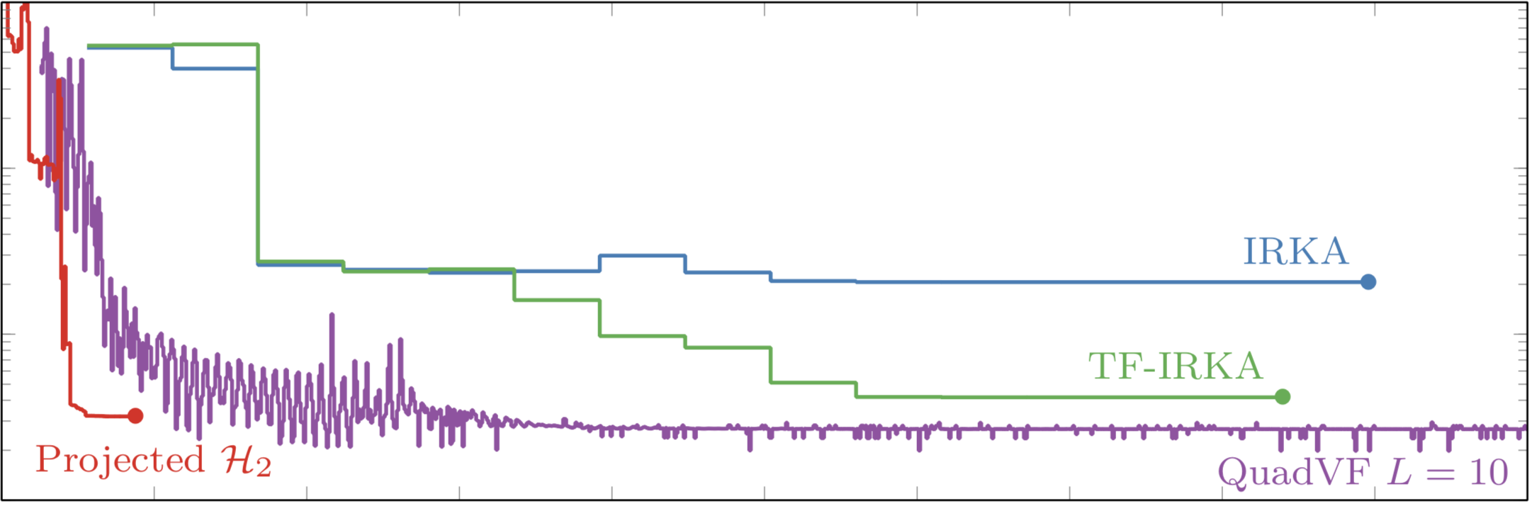
Given access to the transfer function of a linear time-invariant system $H$, model reduction seeks to construct a reduced order model $H_r$ that emulates the dynamics of the full order model. Commonly these reduced order models are choosen to have a real, stable, finite-dimensional state-space form and hence their transfer functions are proper rational functions of degree $r$ whose poles are in the left-half plane; i.e., $H_r \in \mathcal{R}_r(\mathbb{R})^+$. $\mathcal{H}_2$-optimal model reduction seeks the reduce order model that minimizes the $\mathcal{H}_2$-norm: $$ \min_{H_r\in \mathcal{R}_r^+(\mathbb{R})} \| H - H_r \|_{\mathcal{H}_2}^2, \qquad \| F \|_{\mathcal{H}_2}^2 = \int_{-\infty}^\infty |F(i\omega)|^2 \mathrm{d}\omega. $$ By exploiting the Hilbert space structure of this norm, we are able to construct an efficient algorithm that solves the $\mathcal{H}_2$-optimal model order reduction problem by projecting onto a sequence of finite dimensional subspaces, each yielding a least squares rational approximation problem $$ H_r^{\ve\mu^{(k)}} = \argmin_{H_r\in \mathcal{R}_r^+(\mathbb{R})} \| P(\ve\mu_k) [H - H_r]\|_{\mathcal{H}_2}^2. $$
A Data-driven McMillan Degree Lower Bound
Jeffrey M. Hokanson
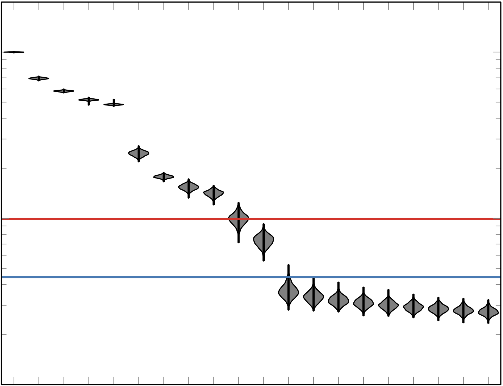
Given measurements of a linear time-invariant system, the McMillan degree is the dimension of the smallest such system that reproduces these observed dynamics. When given impulse response measurements $\lbrace y_j \rbrace_{j=0}^{n-1}$ of the system $\lbrace \ma A, \ve c, \ve x_0\rbrace$, $$ y_j := \ve c^* \ve x_j \quad \ve x_{j+1} := \ma A \ve x_j $$ the McMillan degree is the rank of the Hankel matrix $\ma H$ built from $\lbrace y_j \rbrace_{j=0}^{n-1}$: $$ \ma H = \begin{bmatrix} y_0 & y_1 & \cdots & y_{m-1} \\ y_1 & y_2 & \cdots & y_m \\ \vdots &\vdots & & \vdots \\ y_{n-m-1} & y_{n-m} &\cdots & y_{n-1} \end{bmatrix}. $$ However if $\lbrace y_j \rbrace_{j=0}^{n-1}$ is contaminated by noise, this matrix is almost surely full rank. In this paper we introduce a new upper bound on the rank of a random Hankel matrix and use this bound to construct a lower bound of the McMillan degree.
Data-driven Polynomial Ridge Approximation Using Variable Projection
Jeffrey M. Hokanson and Paul G. Constantine
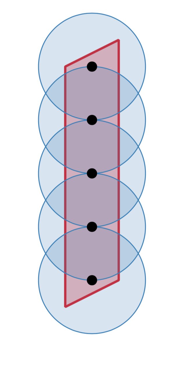
A ridge approximation mimics a scalar function of many variables $f: \R^m\to \R$ by another function $g:\R^n \to \R$ of a few linear combinations of inputs such that $$ f(\ve x) \approx g(\ma U^\trans \ve x) \quad \ma U\in \R^{m\times n} \quad \ma U^\trans \ma U = \ma I. $$ In this paper we find the ridge function $g$ and the subspace spanned by $\ma U$ by minimizing the 2-norm mismatch between $f(\ve x_i)$ and $g(\ma U^\trans \ve x_i)$ over a user provided set of points $\lbrace \ve x_i\rbrace_{i=1}^N$. By assuming $g$ is a multidimensional polynomial, we can implicitly solve for the coefficients using variable projection and solve the remaining optimization problem over the Grassmann manifold of $n$-dimensional subspaces of $\R^m$. The resulting algorithm allows for the rapid construction of ridge approximations using only function values.
Projected Nonlinear Least Squares for Exponential Fitting
Jeffrey M. Hokanson
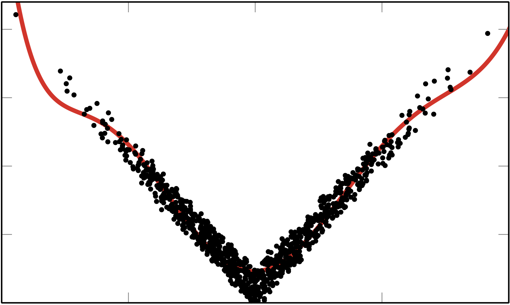
The exponential fitting problem seeks to minimize the mismatch between a noisy vector of measurements $\tve y\in \R^n$ and a sum of complex exponentials in a least squares sense: $$ \minimize_{\ve \omega, \ve a\in \C^p} \| \ve f(\ve\omega, \ve a) - \tve y\|_2^2 \qquad [\ve f(\ve\omega, \ve a)]_k = \sum_{j=1}^p a_j e^{\omega_j k}. $$ To speed optimization when vast quantities of data are present, we project the problem onto a low dimensional subspace $$ \|\ma W \ma W^*\ve f(\ve\omega, \ve a) - \ma W^*\tve y\|_2^2= \|\ma W^*\ve f(\ve\omega, \ve a) - \ma W^*\tve y\|_2^2, \quad \ma W^*\ma W = \ma I. $$ By a careful selection of $\ma W$ that allows us to efficiently evaluate $\ma W^*\ve f(\ve\omega, \ve a)$ we are able to outperform subspace-based approaches for exponential fitting.

One Can Hear the Composition of a String:
Experiments with an Inverse Eigenvalue Problem
Steven J. Cox,
Mark Embree,
and Jeffrey M. Hokanson
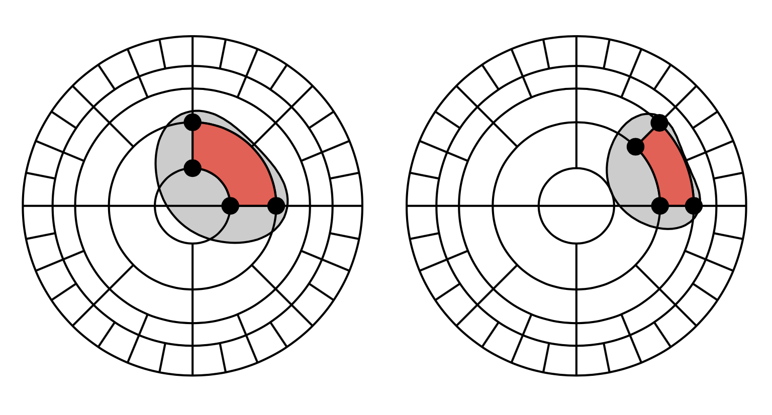
An inverse eigenvalue problem seeks to infer properties of a system through its eigenvalues. A classic example is Kac's question: Can one hear the shape of a drum?; the answer turns out to be no in two dimensions. In this paper we develop a version of this problem accessible to undergraduates in a matrix analysis course. Here we consider the case of a beaded string where the beads are symmetrically distributed around the mid-point of the string. Using classical results of Gantmacher, Krein, and others, we develop an algorithm to recover the masses and locations of these beads given the resonant frequencies of the beaded string. We apply this algorithm to datasets generated from an actual beaded string. This example is used as component of a teaching lab suitable for juniors and above.
Software
Parameter Space Dimension Reduction
The goal of parameter space dimension reduction is to provide a reduced set of coordinates
to approximately describe a function.
Specifically, given a scalar-valued function $f:\set D \subset \R^m \to \R$,
we seek to find a surjective map $h:\set D\to \R^n$ where $n\ll m$ such that
$$ f(\ve x) \approx g(h(\ve x)) \quad \forall \ve x \in \set D, \ g:\R^n\to \R.$$
By identifying $h$ mapping to a lower dimensional space,
the complexity of approximating $f$ no longer grows exponentially in input dimension $m$.
This package includes:
| dimension reduction | |
| response surfaces | |
| test problems | domains | function tools |
Applied Math Laboratory
During the summer of 2007 I was supported by a Brown teaching grant to help build a teaching laboratory to accompany the CAAM department's undergraduate linear algebra class. Together with Steve Cox and Mark Embree I helped devise the experiments and built the accompanying apparatus. Below, I highlight a few of these experiments.
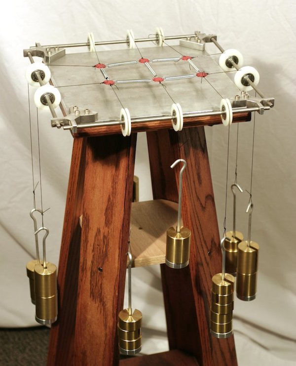
Force table
As part of labs 3 and 4, the students would work with a spring network resembling problems in the course textbook. In lab 3, the students would verify the forward problem: knowing the stiffness of the springs, the topology, and the applied loads they would compute the expected displacement and check that it matched the model. In lab 4, the students would solve the inverse problem: knowing the topology of the spring network and the displacements they would attempt to infer stiffness of each spring.
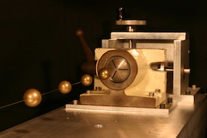
Multiple pendula
In lab 8, the students would recreate the 1733 experiment of Daniel Bernoulli illustrating the superposition of eigenfunctions on a multiple pendula. First the students would displace the each of the masses in an eigenvector, and observe that the motion was always a scalar multiple of the initial displacement. Then the students displace the masses randomly and measure their displacement as a function of time using video tracking software. By taking the discrete Fourier transform of this displacement the students would note the same three resonant frequencies of the pendula seen when the masses were displaced in an eigenvector configuration.
Beaded string
In labs 9 and 10 the students would work with a beaded string. In the first lab, the students would study the forward problem: placing beads on the string knowing their displacement and mass and verify the eigenvalues of the string matched a discrete model In the second lab, the students would place the beads symmetrically around the mid-point of the string and estimate the masses and location of the beads from the measured eigenvalues.